TrajAtlas meets Spatial Omic#
Setup#
Here, we load TrajAtlas software and our gingival atlas datasets.
import TrajAtlas as tja
import scanpy as sc
import numpy as np
import pandas as pd
adata = sc.read("../important_processed_data/4.7_scMerge.h5ad")
adata = adata[:,adata.var["pattern"].dropna().index]
sc.pp.normalize_total(adata, inplace=True)
sc.pp.log1p(adata)
adata.var["pattern"] = "pattern" + adata.var["pattern"].astype("int").astype("str")
/home/zhanglab/mambaforge/envs/py311/lib/python3.11/site-packages/scanpy/preprocessing/_normalization.py:206: UserWarning: Received a view of an AnnData. Making a copy.
  view_to_actual(adata)
You need have following things to check out before you run this pipeline.
The count matrix in adata.X should be normalized.
“Pattern” should be one of your
adata.varslot. The algorithm to find patterns are not emmbeded in TrajAtlas. We recommend you to run with SpatialDE.The value in adata.var.pattern should be in your
adata.obs.columns
adata.X[0:5,0:5].toarray()
array([[0.94, 0.  , 0.  , 0.94, 0.  ],
       [0.  , 0.8 , 0.  , 0.8 , 0.8 ],
       [1.24, 0.  , 0.  , 1.24, 1.24],
       [0.  , 0.  , 0.  , 0.  , 2.46],
       [0.52, 0.86, 0.52, 0.  , 0.  ]])
adata.var["pattern"]
Lypla1      pattern0
Tcea1       pattern5
Rgs20       pattern1
Atp6v1h     pattern7
Rb1cc1      pattern6
              ...
Ankrd34b    pattern7
Kcng3       pattern7
Chrna9      pattern2
Matn3       pattern7
Ak7         pattern6
Name: pattern, Length: 10789, dtype: category
Categories (8, object): ['pattern0', 'pattern1', 'pattern2', 'pattern3', 'pattern4', 'pattern5', 'pattern6', 'pattern7']
adata
AnnData object with n_obs × n_vars = 13056 × 10789
    obs: 'nCount_RNA', 'nFeature_RNA', 'percent.mt', 'orig.ident', 'celltype', 'idents', 'n_genes_by_counts', 'log1p_n_genes_by_counts', 'total_counts', 'log1p_total_counts', 'pct_counts_in_top_50_genes', 'pct_counts_in_top_100_genes', 'pct_counts_in_top_200_genes', 'pct_counts_in_top_500_genes', 'point', 'pattern0', 'pattern1', 'pattern2', 'pattern3', 'pattern4', 'pattern5', 'pattern6', 'pattern7'
    var: 'n_cells_by_counts', 'mean_counts', 'log1p_mean_counts', 'pct_dropout_by_counts', 'total_counts', 'log1p_total_counts', 'pattern', 'membership'
    uns: 'log1p'
    obsm: 'spatial'
    layers: 'logcounts'
Statical test#
In this step, we align the genes to the gene pattern axis, and calculate correlation, expression and peak. Because there are three groups, we use ANOVA to find differential genes. And we also applied boostrap to increase statical power.
sc.pl.embedding(adata,color=['pattern0', 'pattern1', 'pattern2'],basis="spatial",size=70)

Here, we set bootstrap_iterations to be 3. You can increase this number, based on your need.
mdata = utils.getAttributeGEP(adata,sampleKey ="orig.ident",bootstrap_iterations = 3,njobs=20)
Processing Samples: 100%|██████████| 6/6 [00:18<00:00,  3.06s/it]
/home/gilberthan/anaconda3/envs/py311/lib/python3.11/site-packages/pandas/core/internals/blocks.py:393: RuntimeWarning: invalid value encountered in sqrt
  result = func(self.values, **kwargs)
/home/gilberthan/anaconda3/envs/py311/lib/python3.11/site-packages/mudata/_core/mudata.py:491: UserWarning: Cannot join columns with the same name because var_names are intersecting.
  warnings.warn(
mdata
MuData object with n_obs × n_vars = 18 × 9078
  3 modalities
    corr:	18 x 10789
      obs:	'sample', 'bootstrap'
      layers:	'raw', 'mod'
    expr:	18 x 10789
      obs:	'sample', 'bootstrap'
      layers:	'raw', 'mod'
    peak:	18 x 10789
      obs:	'sample', 'bootstrap'
      layers:	'raw', 'mod'
design = {'sample' : ['D0','D0_K5_GFP', 'D3', 'D3_K5_GFP','D5', 'D5_K5_GFP'],
          'group': ["D0","D0","D3","D3","D5","D5"],
         "batch" : ["batch1", "batch2", "batch1", "batch2", "batch1", "batch2"]}
design = pd.DataFrame(design)
design=design.set_index("sample")
mdata["corr"].obs["group"]=np.array(design.loc[mdata["corr"].obs["sample"]]["group"])
This step return you a statical test dataframe. Here, we select ‘P-value_corrected’ < 0.01 as differential genes.
anovadf = utils.attrANOVA(mdata["corr"],group_labels = mdata["corr"].obs["group"])
sigGene = anovadf.Feature[anovadf['P-value_corrected']<0.01]
Visualization#
In this section, we ultilized two way to visualize these differnetial genes.
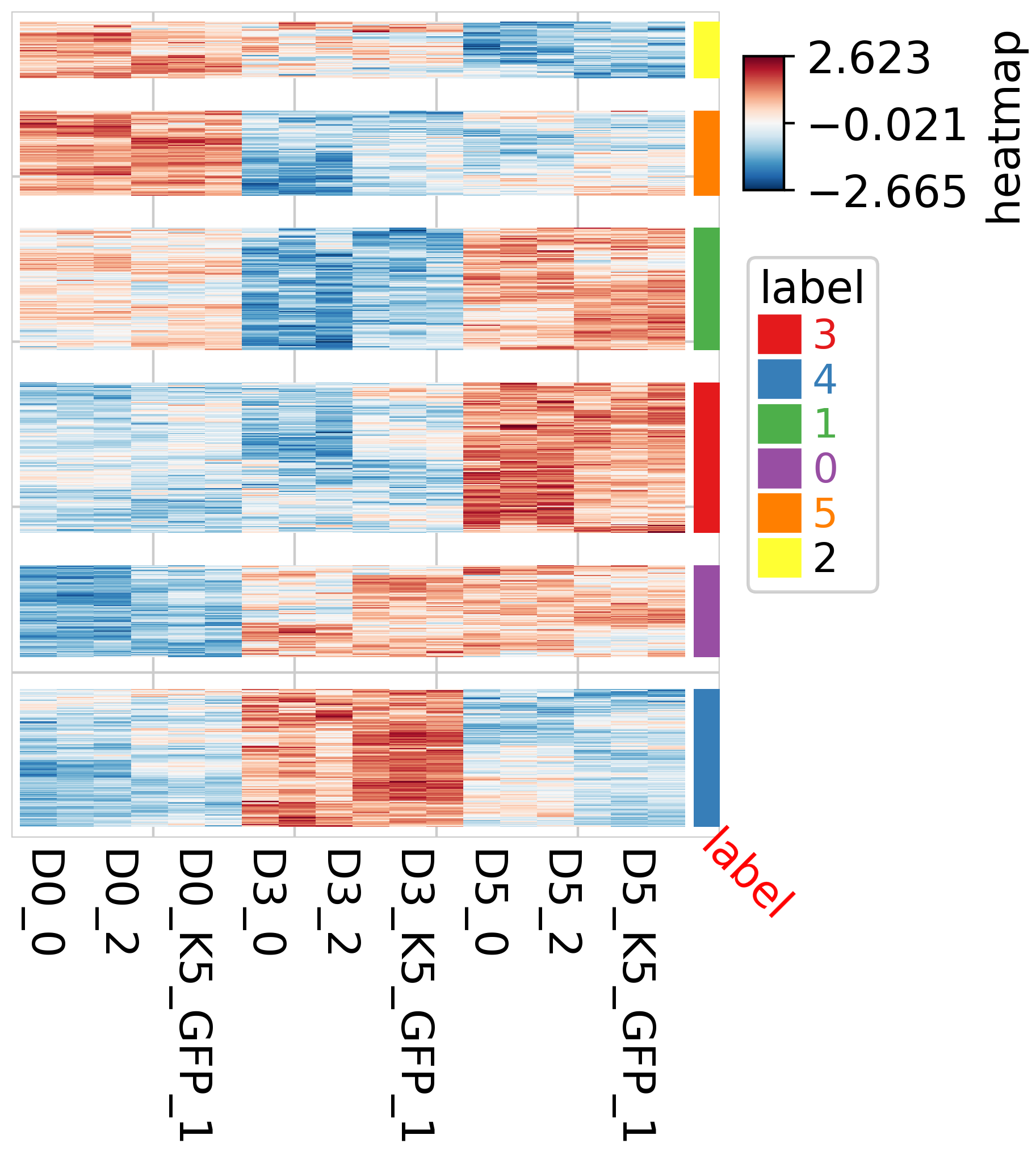
Heatmap, where color represents correlation
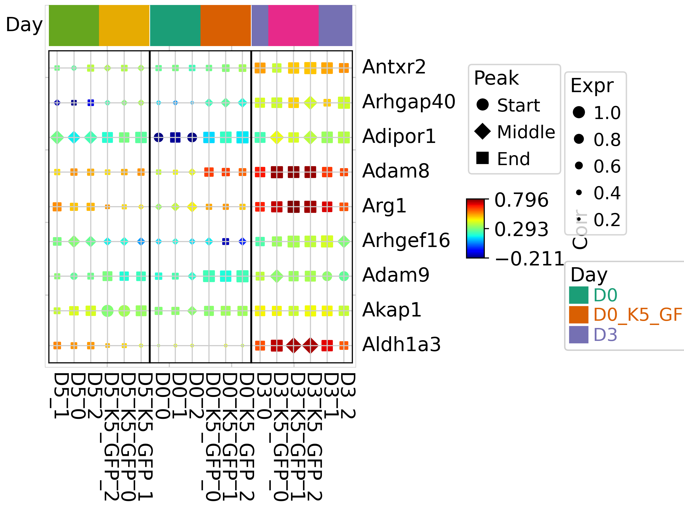
Dotplot, where color represents correlation, size represents expression level, and shape represents peak.
corrDf = pd.DataFrame(mdata["corr"].X)
corrDf.index = mdata["corr"].obs_names
corrDf.columns = mdata["corr"].var_names
corrDf = corrDf.T
sigGene = np.intersect1d(corrDf.index,sigGene)
def z_scale_row(row):
    return (row - row.mean()) / row.std()

# Apply the z-scaling function to each row of the DataFrame
scaled_df = corrDf.apply(z_scale_row, axis=1)
scaled_df = scaled_df.loc[sigGene]
scaled_df.shape
(659, 18)
from sklearn.cluster import KMeans

# Specify the number of clusters
num_clusters = 6

# Initialize the KMeans model
kmeans = KMeans(n_clusters=num_clusters)

# Fit the model to the data
kmeans.fit(scaled_df)

# Get the cluster labels
labels_filter = kmeans.labels_

labels_filter=labels_filter.astype("str")

labels_filter=pd.DataFrame(labels_filter)
labels_filter.index= scaled_df.index
/home/gilberthan/anaconda3/envs/py311/lib/python3.11/site-packages/sklearn/cluster/_kmeans.py:1416: FutureWarning: The default value of `n_init` will change from 10 to 'auto' in 1.4. Set the value of `n_init` explicitly to suppress the warning
  super()._check_params_vs_input(X, default_n_init=10)
import PyComplexHeatmap as pch
import matplotlib.pyplot as plt
row_ha =pch.HeatmapAnnotation(label=labels_filter,
                           label_side='bottom',
                           label_kws={'rotation':-45,'color':'red'},
                           axis=0)
pch.ClusterMapPlotter(scaled_df,show_colnames=True,col_cluster=False,row_split=labels_filter,
                      cmap="RdBu_r",row_split_gap=3,right_annotation=row_ha)
Starting plotting..
Starting calculating row orders..
Reordering rows..
Starting calculating col orders..
Reordering cols..
Plotting matrix..
Starting plotting HeatmapAnnotations
Collecting legends..
Collecting annotation legends..
Plotting legends..
Estimated legend width: 17.767277777777778 mm


<PyComplexHeatmap.clustermap.ClusterMapPlotter at 0x761a91933310>
gene_to_show = labels_filter.index[labels_filter[0] == "4"][1:10]
dotDf = tja.utils.makeDotTable(mdata,gene_to_show,sample= scaled_df.columns)
anno_df
| sample | bootstrap | group | |
|---|---|---|---|
| D0_0 | D0 | 0 | D0 |
| D0_1 | D0 | 1 | D0 |
| D0_2 | D0 | 2 | D0 |
| D0_K5_GFP_0 | D0_K5_GFP | 0 | D0 |
| D0_K5_GFP_1 | D0_K5_GFP | 1 | D0 |
| D0_K5_GFP_2 | D0_K5_GFP | 2 | D0 |
| D3_0 | D3 | 0 | D3 |
| D3_1 | D3 | 1 | D3 |
| D3_2 | D3 | 2 | D3 |
| D3_K5_GFP_0 | D3_K5_GFP | 0 | D3 |
| D3_K5_GFP_1 | D3_K5_GFP | 1 | D3 |
| D3_K5_GFP_2 | D3_K5_GFP | 2 | D3 |
| D5_0 | D5 | 0 | D5 |
| D5_1 | D5 | 1 | D5 |
| D5_2 | D5 | 2 | D5 |
| D5_K5_GFP_0 | D5_K5_GFP | 0 | D5 |
| D5_K5_GFP_1 | D5_K5_GFP | 1 | D5 |
| D5_K5_GFP_2 | D5_K5_GFP | 2 | D5 |
anno_df = mdata["corr"].obs
col_ha = pch.HeatmapAnnotation(
                           Day=pch.anno_simple(anno_df,cmap='Dark2',legend=True,add_text=False),
                           verbose=0,label_side='left',label_kws={'horizontalalignment':'right'})
tja.utils.trajDotplot(dotDf, show_colnames=True,top_annotation = col_ha,spines=True,col_split = anno_df.group)
Starting plotting..
Starting calculating row orders..
Reordering rows..
Starting calculating col orders..
Reordering cols..
Plotting matrix..
Warning: ratio is deprecated, please use max_s instead
Using user provided max_s: 60
Collecting legends..
Plotting legends..
Estimated legend width: 29.5811 mm
Incresing ncol
Incresing ncol
More than 3 cols is not supported
Legend too long, generating a new column..
Incresing ncol